The system identification workflow
Before a MIMO vibration test can be controlled, the controller has to know the plant: drive every shaker with known excitation, measure every response, and estimate the FRF matrix between them. A system ID run is that measurement — and the three readings that decide whether it can be trusted: the FRFs themselves, the multiple coherence that says how much of each response the drives account for, and the signal-to-noise that says how far the excitation stood above the ambient.
The walkthrough is the demonstration plate's system ID — four shakers
into eight response channels, an ambient recording first and the driven one
after — streamed by the controller
(generate_plate_sysid.py in the generators repository) to
stressdata/plate/sysid_stream.nc4.
| Step | In the app | In a script |
|---|---|---|
| Import the stream | drag the .nc4 on; answer yes to the question |
project.import_file(path) |
| Say what it is | (the question did) or Set Project Type → System ID | project.project_type = 'System ID' |
| The FRFs | Compute FRFs in the averaging view — H1 | project.compute_frfs(name, 'H1') |
| Trust, part one | Compute Multiple Coherence | project.compute_multiple_coherence(name) |
| Trust, part two | PSDs of both phases; select the pair; Signal to noise (dB) or RMS signal to noise | project.compute_psds(...) twice, then plot.plot_ratio(...) or plot.plot_snr(...) |
| Geometry and photos | drag them in, link them | project.add(...), project.link(...) |
| Report | Generate Report on the bar, the project row selected | project.generate_report('sysid') |
| Or all of it at once | Automatic on the tree bar, once the project has its type | project.work_up() |
| Save | Save Project As… | project.save('sysid.vdyn') |
In the app, step by step
1. Import the stream, and answer the question
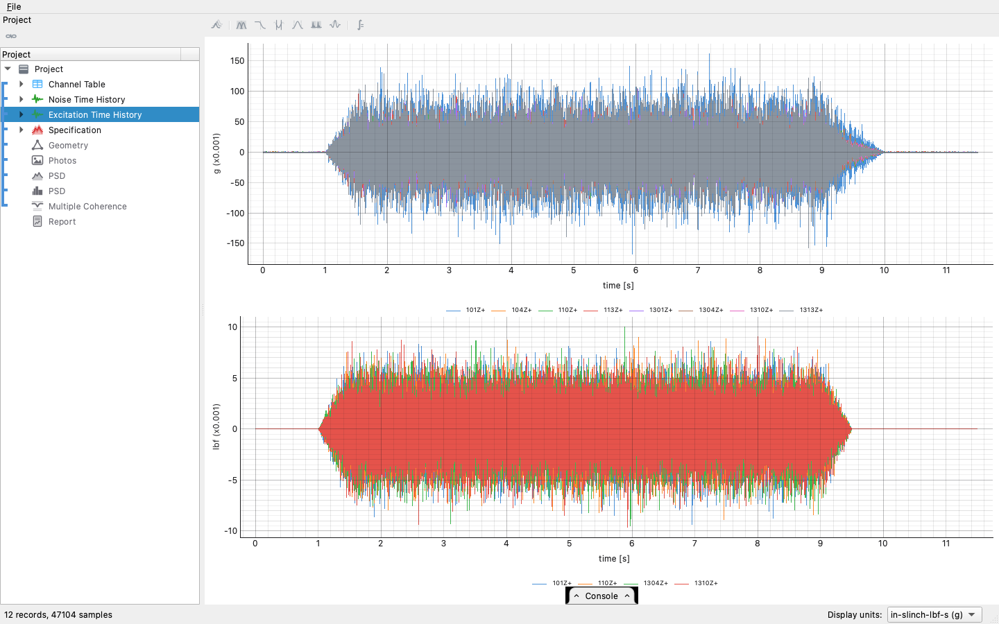
A streamed system ID save is two time streams, a quiet one then a loud one — and at the file level that is indistinguishable from an ordinary run of the same environment. So the app asks rather than guesses: importing a file of that shape poses "Treat this project as a System ID test?", and on yes the two streams take their phase names — Noise Time History for the ambient, Excitation Time History for the driven — told apart by level. (A project already typed System ID is not asked; the streams are named directly. A stop-and-restart run whose two streams are both loud is not asked either.)
2. The FRFs — H1, and why
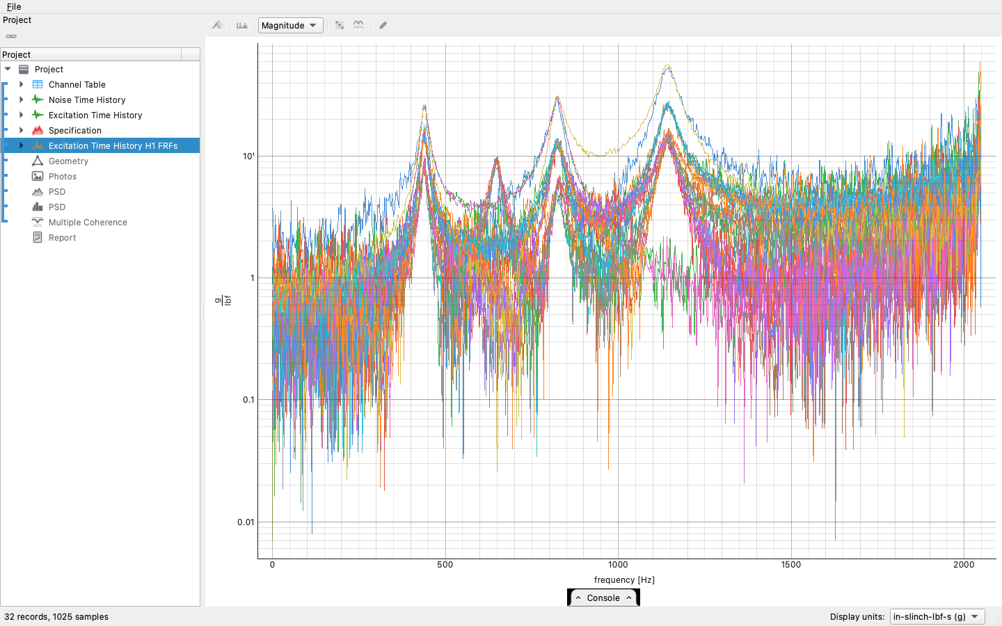
Compute FRFs in the excitation history's averaging view, method
H1: the plant is measured driving through known excitation, so
the noise is on the response side, which is exactly the assumption H1
makes. This is the estimator the controller itself uses for the same
measurement. The drives are the channels whose role is ref in the
history's Role column — the channels the file says were driven —
and a channel marked mon is in no FRF (the tree).
3. Trust, part one: multiple coherence
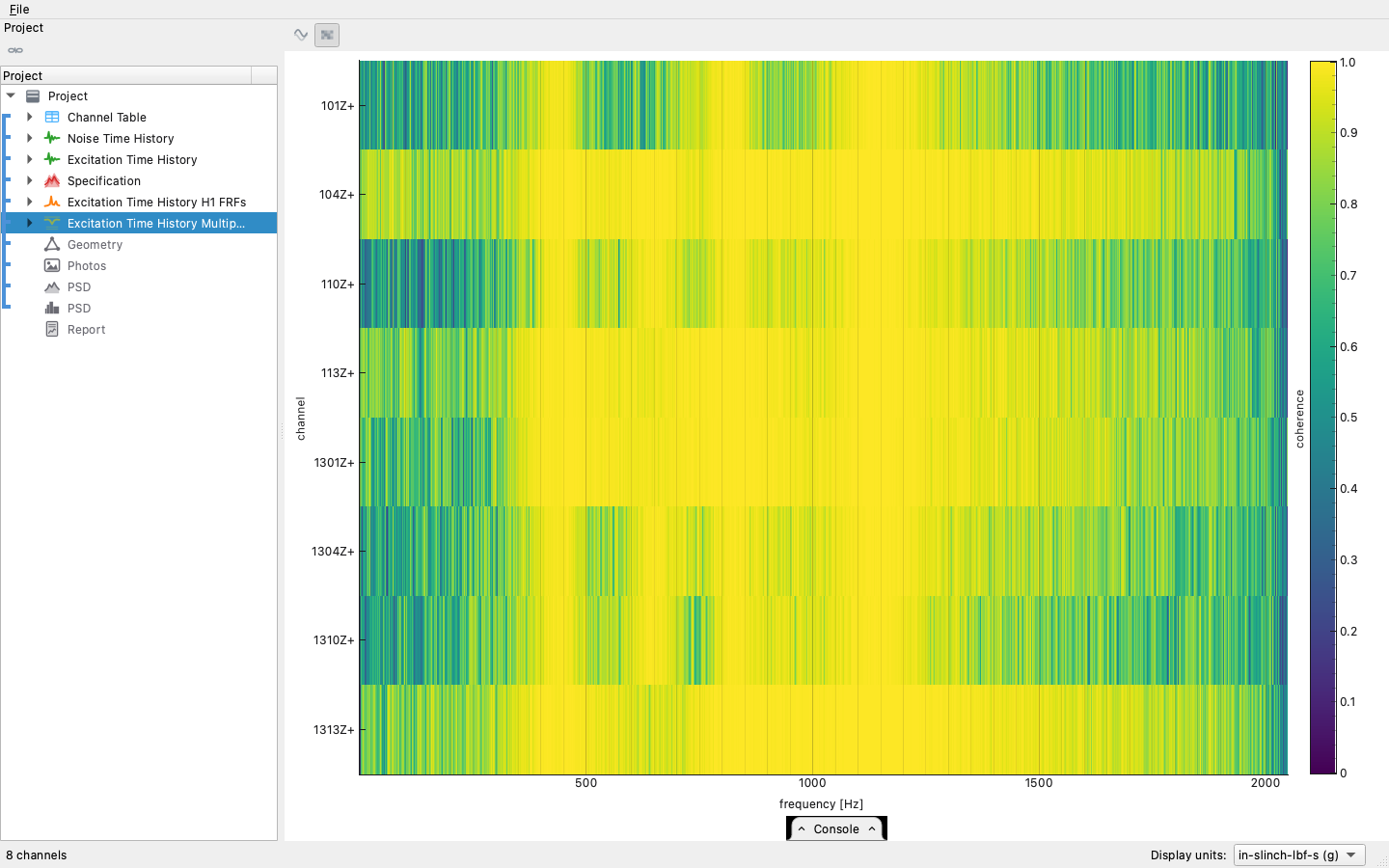
Multiple Coherence, beside it in the same view, reads how much of each response all the drives together account for, line by line. A dip says the response contains something the drives did not put there — a rattle, ambient bleed, a nonlinearity — at exactly those frequencies, and an FRF line under a coherence dip is a line the control law will be inverting on faith.
4. Trust, part two: the signal-to-noise reading
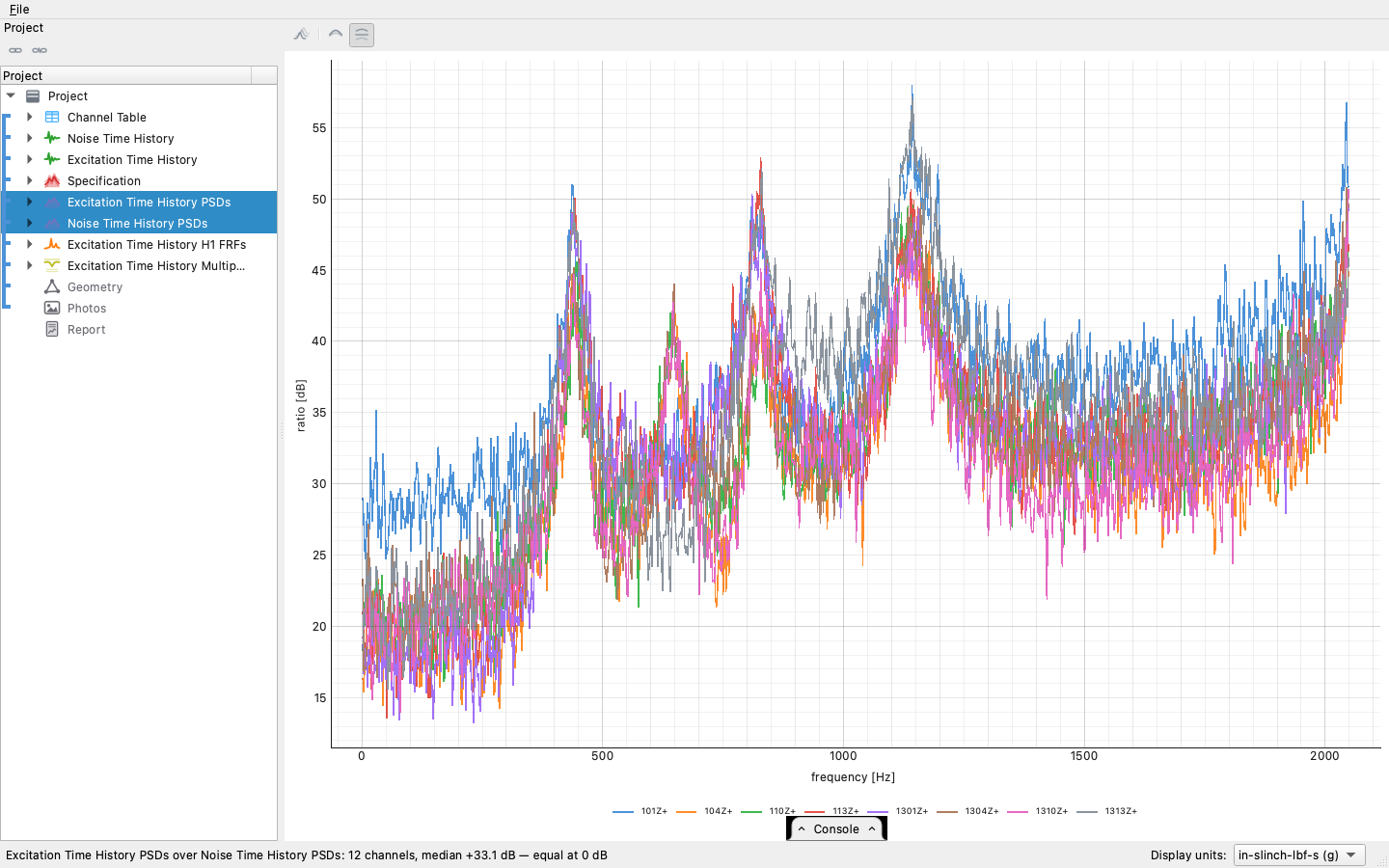
Compute PSDs of both phases, with the ambient borrowing the excitation's frames, since the two densities can only be compared on the same frequency lines. Then select the two PSDs together. The signal-to-noise is a reading of that pair, never a third object, and the bar offers it two ways:
- Signal to noise (dB) draws one curve per channel, line by line. Where the excitation stood 30 dB over the ambient, the FRF there is a measurement. A line with nothing above the ambient is not drawn.
- RMS signal to noise draws one bar per channel, the same ratio taken over the whole band. Channels under the threshold, 10 dB to start, are colored, and the threshold can be dragged. A channel with no signal above its noise has no bar and is labeled as at the noise floor. A channel whose ambient recorded nothing is left off, and the status line says how many.
How both are computed, and the definition they follow, is in How the signal-to-noise is computed.
5. Geometry, photos, report
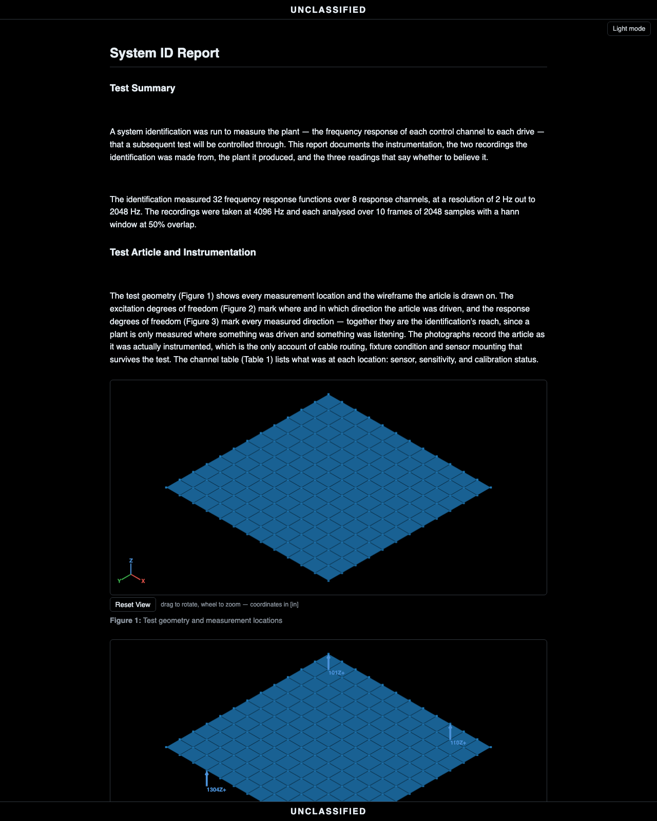
Drag the article's geometry in, declare its units, add the setup photographs, link the group. The system ID report binds both recordings with their frames, the excitation and ambient densities overlaid per channel, the FRF magnitudes, the multiple coherence as a map (frequency across, channel down), the signal-to-noise per channel, the RMS signal-to-noise bars, and the kurtosis of each recording — the record a control run stands on. Every figure in it is 2-D, as in the random and sine reports: the 3-D stage made the files too large. A figure of more than two dozen curves continues into further figures rather than leaving channels out.
The same run, headless
And the script never has to be reconstructed by hand: the console tab along the bottom of the window writes it live as you click — every act of the session as the line that replays it. Expand it, copy the stretch you want, and it runs as-is.
The whole thing is one call when the defaults are right:
It asks for what it is not given, exactly as
the random vibration report does. Called with no
run it opens a file dialog, takes as many recordings as are chosen and
writes one report each; a run chosen that way is asked once for a
geometry to share across the batch, where Cancel means none. path
may be the file to write or a folder each report lands in under its
run's own name.
visualdynamics.system_id_report()                  # ask for both
visualdynamics.system_id_report(path='reports/')   # ask, write here
visualdynamics.system_id_run is the same workup stopping at the
project, for when it should live on — to save as .vdyn, or to read
the plant against something else.
import numpy as np

import visualdynamics

project = visualdynamics.Project('Plate System ID')

# 1. import; a script is never asked, so the type is declared and the
# two phases are named for what they are, quiet first
project.import_file('sysid_stream.nc4')
project.project_type = 'System ID'
histories = sorted(
    (name for name in project.names
     if type(project[name]).__name__ == 'TimeHistory'),
    key=lambda name: float(np.asarray(project[name].ordinate).std()))
project.rename(histories[0], 'Noise Time History')
project.rename(histories[1], 'Excitation Time History')

# 2. geometry, photos, links
geometry = visualdynamics.import_file('geometry.npz')
geometry.define_units('m')
project.add('Geometry', geometry)
project.link(*project.names)
project.set_basis(*project.names)

# 3. the plant, and the two trust readings
project.compute_frfs('Excitation Time History', 'H1')
project.compute_multiple_coherence('Excitation Time History')
project.compute_psds('Excitation Time History')
project['Noise Time History'].averaging = \
    project['Excitation Time History'].averaging
project.compute_psds('Noise Time History')

# 4. report and save
project.generate_report('sysid')
project.export_report(project.report, 'sysid_report.html')
project.save('sysid.vdyn')
How the signal-to-noise is computed
Signal-to-noise ratio is the power of the signal over the power of the noise. The definition is the standard one, used for digitizers in IEEE Std 1241 and for random data by Bendat and Piersol (Random Data: Analysis and Measurement Procedures, 4th ed., Wiley, 2010).
A system identification does not record the signal alone. The ambient recording is the noise \(N\): the room, the amplifiers, the cabling and the sensors, with the drives at zero. The driven recording is the signal plus that same noise. When the noise is uncorrelated with the signal, their powers add, so the signal's power is the driven power less the ambient power. At each frequency line \(f\), with \(G_d\) the driven autospectral density and \(G_n\) the ambient one,
The RMS signal-to-noise of a channel uses the mean-square value of each recording over the band the two densities share, which is the area under the density, \(P = \int G(f)\,df\), integrated the way the density is drawn:
The plain quotient \(G_d / G_n\) is \(\mathrm{SNR} + 1\). The two agree when the margin is large and differ near the noise floor:
| Driven over ambient | Signal to noise |
|---|---|
| 3 dB | 0 dB |
| 6 dB | 4.8 dB |
| 10 dB | 9.5 dB |
| 20 dB | 19.96 dB |
Visual Dynamics used the plain quotient through 0.1.0a33. It reads high on exactly the channels the reading is meant to find, so both the curve and the bars now use the subtracted form.
Where the driven power does not exceed the ambient, there is no signal to state. That happens on a channel the drives never reached, and on single lines where estimation scatter puts the driven density under the ambient one. The curve leaves those lines out, and the bars give the channel no number, label it as at the noise floor, and count it under the threshold.
A line or channel whose ambient recorded exactly zero is a different case. On hardware that is noise below the recording's resolution, and in a simulation a quiet that was exactly silent. There is no noise to divide by, so the curve leaves the line out, and the bars leave the channel out and say how many channels that was. A simulated drive point's load cell, whose ambient is silent, would otherwise be flagged as the worst channel when it is the cleanest.
The same quantity sets the threshold. With the noise on the response, the ordinary coherence between drive and response is \(\gamma^2 = \mathrm{SNR} / (1 + \mathrm{SNR})\) (Bendat and Piersol). At 10 dB that is 0.91, about where a coherence is usually required to be, so the bars start their threshold at 10 dB.
The RMS value is a summary. It is dominated by the frequencies where the power is, and a channel can read 30 dB over the band while sitting on its noise floor across part of it. The bars rank the channels, and the curve shows where in the band a channel was weak.
The two recordings also answer a narrower question than the coherence does. The ambient recording measures the noise of the measurement chain. The multiple coherence measures everything in the response the drives do not account for, which also includes rattles, nonlinearity and inputs that were not measured. That is why the report shows both.
Where judgment lives
- The question at import is a question because the file cannot answer it. Two streams, quiet then loud, is also what a stop-and-restart run leaves. The 10 dB gate keeps the obvious non-cases from asking, but the yes is the engineer's.
- Which save to work from. The controller also writes a spectral package — the measured FRFs, coherence and autospectra it computed itself. That imports directly, but it records hardware channel numbers with no units; the stream carries the channel table, so everything computed from it wears real node labels and engineering units and links to the geometry. When both exist, work from the stream and keep the package as the controller's own cross-check.
- A drive with no noise floor reads NaN. The signal-to-noise of a drive channel divides the drive by an ambient that recorded silence, and there is no ratio to state rather than an infinite one. Those lines are not drawn, and the bars leave the channel out and count it in the caption.
- Coherence near one is necessary, not sufficient. It says the responses are linearly explained by the drives — it does not say the levels were right for the article, which is what the signal-to-noise reading is for. The two together are the case for trusting the plant; neither alone is.